A correlation analysis provides the necessary information on the strength and direction of the linear relationship between x and y. For assessing the correlation between numeric variable the Pearson correlation coefficient r, is used, and can take values between -1 and 1. Zero resides in the middle of this interval and stands for no relationship. The further away from zero the stronger the relationship. The sign of r indicative of the relationship between the variables. If r is positive, then as one variable increases, the other also behaves in the same way (increase). The opposite is true when the sign is negative.
The correlation coefficient can be found using the following formula:
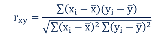
Where:
- rxy – the correlation coefficient of the linear relationship between the variables x and y
- xi – the values of the x-variable in a sample
- x̅ – the mean of the values of the x-variable
- yi – the values of the y-variable in a sample
- ȳ – the mean of the values of the y-variable
Lets turn to R to dive in some examples using a dataset with some biomechanical features of the vertebral column found in UCI machine learning repository
# Reorder the correlation matrix
spinecor <- arrange_spinecor(spinecor)
upper_tri <- get_upper_tri(spinecor)
# Turn the correlation matrix into long format
longspinecor1 <- melt(upper_tri, na.rm = TRUE)
# Create a heatmap with ggglot
suppressMessages(library(viridis))
ggheatmap <- ggplot(longspinecor1, aes(Var2, Var1, fill = value))+
 geom_tile(color = "white")+
 scale_fill_viridis(option='magma',limit = c(-1,1), space = "Lab",
    name="Pearson\nCorrelation") +
 theme_minimal()+ # minimal theme
 theme(axis.text.x = element_text(angle = 45, vjust = 1,
                                  size = 12, hjust = 1))+
 coord_fixed()+geom_text(aes(Var2, Var1, label = value), color = "black",  size = 4) +
theme(axis.title.x = element_blank(),
  axis.text.x = element_text(angle=45,size = 10),
  axis.text.y = element_text(size = 10),
  axis.title.y = element_blank(),
  panel.grid.major = element_blank(),
  panel.border = element_blank(),
  panel.background = element_blank(),
  axis.ticks = element_blank(),
  legend.justification = c(1, 0),
  legend.position = c(0.6, 0.7),
  legend.direction = "horizontal")+
  guides(fill = guide_colorbar(barwidth = 7, barheight = 1,
                               title.position = "top", title.hjust = 0.5))
# Print the heatmap
print(ggheatmap)
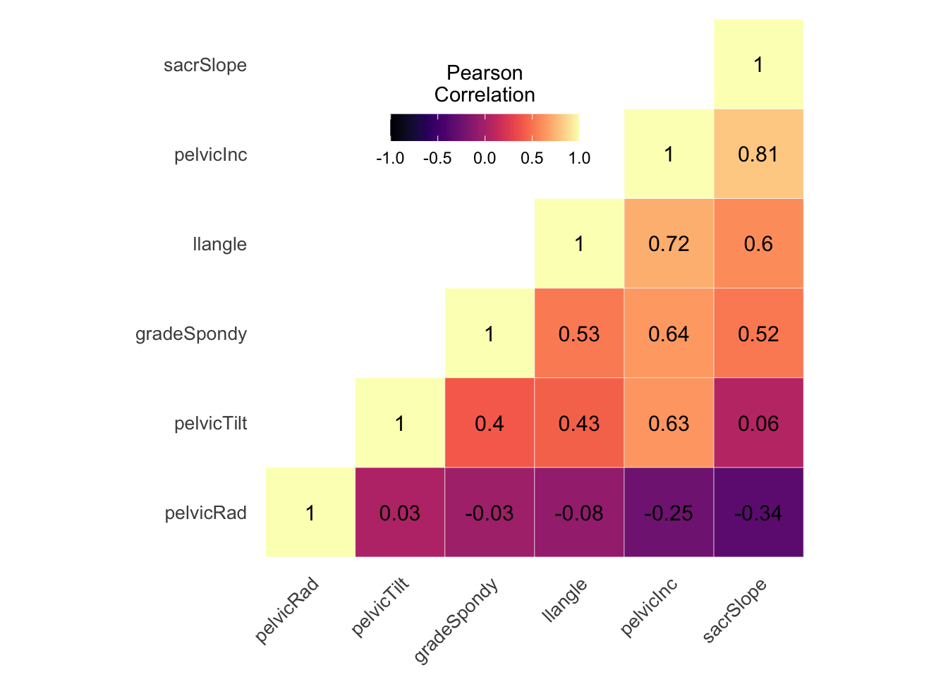
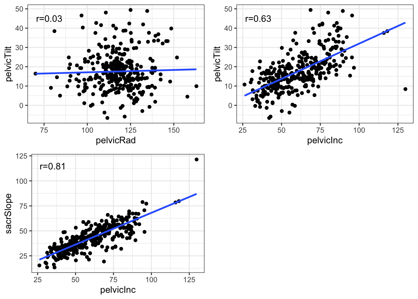
Now that we estimated the strength of the linear associations between our variables let’s how they will depict in a scatterplot.The fit of the data can be visually represented with a scatterplot. Using that plot, we can generally assess the relationship between the variables and determine whether they are correlated or not.
suppressMessages(library(gridExtra))
#no association
g1=ggplot(spine,aes(pelvicRad,pelvicTilt))+geom_point()+theme_bw()+
  annotate('text',x=78,y=45,label='r=0.03')+geom_smooth(method = 'lm',se=F)
#moderate association
g2=ggplot(spine,aes(pelvicInc,pelvicTilt))+geom_point()+theme_bw()+
  annotate('text',x=35,y=45,label='r=0.63')+geom_smooth(method = 'lm',se=F)
#high association
g3=ggplot(spine,aes(pelvicInc,sacrSlope))+geom_point()+theme_bw()+
  annotate('text',x=35,y=115,label='r=0.81')+geom_smooth(method = 'lm',se=F)
grid.arrange(g1,g2,g3,ncol=2)
## `geom_smooth()` using formula 'y ~ x'
## `geom_smooth()` using formula 'y ~ x'
## `geom_smooth()` using formula 'y ~ x'
For those who want to calculate the r coefficient by hand the workflow is: n order to calculate the correlation coefficient using the formula above, you must undertake the following steps:
- Find a data sample with values for x and y variables.
- Calculate the means x̅ for the x-variable and ȳ for the y-variable.
- For the x, subtract the mean from each value of the x-variable (lets call this new variable a). Do the same for the y (lets call this variable b).
- Multiply each a by the corresponding b and calculate the sum of these multiplications (the final value is the numerator in the equation).
- Square each a and sum the result.
- Find the square root of the value obtained in the previous step (this is the denominator in the formula).
- Divide the value obtained in step 4 by the value obtained in step 7.